Sensitivity Testing

The spatiotemporal DBSCAN procedure we use to create our AR catalog involves several hyperparameters. The final choices of these hyperparameters were largely motivated by our physical understanding of ARs in Antarctica (background domain knowledge), and verified ‘by-eye’ by tracking down known ARs from numerous case studies in the Antarctic AR literature and checking that their landfalling time, duration, etc. matches what we found in our catalog. However, there are several perturbations to these parameters that we could have made, and this notebook documents the sensitivity of various AR metrics to these perturbations, conveying the overall importance of getting certain hyperparameters “right.”

Hyperparameters Overview¶

In the clustering algorithm, there are several hyperparameters:

epsilon_space: spatial neighborhood, given in fractions of synoptic scale (1000 km)
epsilon_time: time neighborhood, given in hours
minpts: the minimum number of neighboring points to be considered a core point
n_rep_pts: the number of representative points to sample from each cluster at each time step

In the below sections, we explore the sensitivity of the clustering results to each of these hyperparameters. In our explorations and ground-truthing exercises, we found that an ideal set of hyperparameters are epsilon_space: 0.5, epsilon_time: 12, minpts: 5, and n_rep_pts: 10. We will perturb these hyperparameters individually and explore how they affect clustering results relative to this base setting.

import pandas as pd
import xarray as xr
import matplotlib.pyplot as plt
import os
import sys
from pathlib import Path
import seaborn as sns
from huggingface_hub import login # used to download catalogs with perturbed hyperparams

from artools.display_utils import display_catalog
from artools.loading_utils import load_catalog

First, we define the following helper function, which we will use to process and compute counts of landfalling ARs in catalogs constructed with perturbed values of a hyperparameter of interest.

def process_cts(dictionary):
    '''
    A simple helper function that takes in a dictionary mapping hyperparameter variations
        (deviations from the default/official set) to the respective catalog in pd.DataFrame
        format, and computes landfalling storm counts.
    '''

    res_dict = {}
    total_cts = []
    landfall_cts = []
    for param, df in dictionary.items():
        landfalling = df[df.is_landfalling]
        total_cts.append(df.shape[0])
        landfall_cts.append(landfalling.shape[0])

    res_dict = {'total': total_cts, 'landfalling': landfall_cts}
    res_df = pd.DataFrame(res_dict, index=list(dictionary.keys()))

    return res_df

login()

We first load up the catalog with the official set of parameters. In the rest of the notebook, we go through each hyperparameter and vary that particular hyperparameter relative to the original setting. So, each hyperparameter is only varied individually, not together.

baseline_df = load_catalog('epsspace0.5_epstime12_minpts5_nreppts10_seed12345.h5')

`epsilon_space` perturbations¶

We first perturb the $\epsilon_{space}$ parameter. This parameter is represented as fractions of synoptic scale, or fractions of 1000 km.

# constructing dictionaries to organize results
space_dict = {}
space_dict['0.5'] = baseline_df
space_dict['0.25'] = load_catalog('epsspace0.25_epstime12_minpts5_nreppts10_seed12345.h5')
space_dict['0.75'] = load_catalog('epsspace0.75_epstime12_minpts5_nreppts10_seed12345.h5')
space_dict['1.0'] = load_catalog('epsspace1.0_epstime12_minpts5_nreppts10_seed12345.h5')

res_df = process_cts(space_dict)
res_df

To better assess the sensitivity of storm counts to hyperparameter perturbations, relative to the storm counts of the official configuration, we also compute the percent difference between storm counts of catalogs with the perturbed hyperparameters and the official catalog.

# percent difference, expressed as a percentage of the total number of storms in baseline configuration
space_percents = (res_df - res_df.loc['0.5'])/res_df.loc['0.5']
space_percents

We also visualize the percent differences.

sns.barplot(data=space_percents, x=space_percents.index, y='landfalling', errorbar=None);
plt.axhline(y=0, linestyle='-', color='black')
plt.title('Landfalling AR Counts, Eps. Space')
plt.xlabel('Eps. Space')
plt.ylabel('% Difference');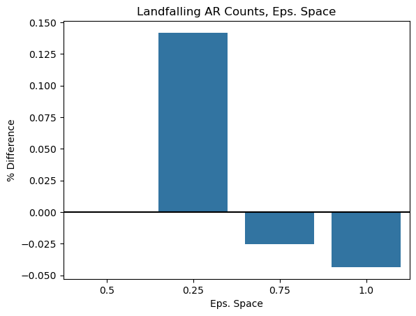

Takeaway: Higher spatial epsilons lead to less ARs, which makes sense as ARs that are close to one another in the same time step are more likely to be grouped together. However, once you are at half a synoptic scale (0.5), the percent difference in the number of landfalling ARs is relatively small. It also appears that the total number of ARs is more sensitive to these perturbations. 0.25 has substantially more landfalling ARs, but this is much too small as groups of AR points within this small distance (250 km) are likely part of the same system.

`epsilon_time` perturbations¶

We next move on to perturbing the $\epsilon_{time}$ parameter. This parameter is expressed in units of hours, and represents how far into the future and past we will look for candidate neighboring points in our clustering algorithm.

# constructing dictionaries to organize results
time_dict = {}
time_dict['9'] = load_catalog('epsspace0.5_epstime9.0_minpts5_nreppts10_seed12345.h5')
time_dict['12'] = baseline_df
time_dict['15'] = load_catalog('epsspace0.5_epstime15.0_minpts5_nreppts10_seed12345.h5')
time_dict['18'] = load_catalog('epsspace0.5_epstime18.0_minpts5_nreppts10_seed12345.h5')
time_dict['21'] = load_catalog('epsspace0.5_epstime21.0_minpts5_nreppts10_seed12345.h5')
time_dict['24'] = load_catalog('epsspace0.5_epstime24.0_minpts5_nreppts10_seed12345.h5')

res_df = process_cts(time_dict)
res_df

# percent difference, expressed as a percentage of the total number of storms in baseline configuration
time_percents = (res_df - res_df.loc['12'])/res_df.loc['12']
time_percents

sns.barplot(data=time_percents, x=time_percents.index, y='landfalling', errorbar=None);
plt.axhline(y=0, linestyle='-', color='black')
plt.title('Landfalling AR Counts, Eps. Time')
plt.xlabel('Eps. Time')
plt.ylabel('% Difference');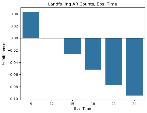

Takeaway: This parameter seems to be consistently impacting the number of landfalling and total numbers of ARs. As before, it seems the total number of ARs is more sensitive to these perturbations. When searching for neighboring points, this parameter represents the time window where we can consider other points to potentially be a part of this same cluster. Anything higher than 18 hours seems too long, since if an AR disappears for 18 hours, it is likely another system. A well-accepted threshold for stitching ARs temporally is 12 hours, as employed in Maclennan et al. (2023) and the definition of cloud-mass meridional transport events.

`minpts` perturbations¶

We also vary minpts, or the minimum number of points that must be in a neighborhood of another point for that point to be considered a core point, and potentially instantiate its own cluster if it isn’t already part of one.

minpts_dict = {}
minpts_dict['3'] = load_catalog('epsspace0.5_epstime12_minpts3_nreppts10_seed12345.h5')
minpts_dict['5'] = baseline_df
minpts_dict['8'] = load_catalog('epsspace0.5_epstime12_minpts8_nreppts10_seed12345.h5')
minpts_dict['10'] = load_catalog('epsspace0.5_epstime12_minpts10_nreppts10_seed12345.h5')

res_df = process_cts(minpts_dict)
res_df

# percent difference, expressed as a percentage of the total number of storms in baseline configuration
minpts_percents = (res_df - res_df.loc['5'])/res_df.loc['5']
minpts_percents

sns.barplot(data=minpts_percents, x=minpts_percents.index, y='landfalling', errorbar=None);
plt.axhline(y=0, linestyle='-', color='black')
plt.title('Landfalling AR Counts, Min. Pts.')
plt.xlabel('Min. Pts.')
plt.ylabel('% Difference');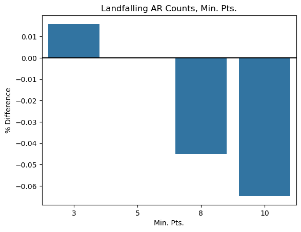

Takeaway: It’s unsurprising that the higher the min_pts parameter, the less storms you get since you require more points witihn a neighborhood of each other to instantiate a cluster. The differences don’t seem that substantial, but 5 intuitively makes sense given the spatiotemporal clustering step works by stitching groups of 10 points from each cluster across time.

`n_rep_pts` perturbations¶

After identifying the clusters present within each time step, we sample a random set of representative points from each cluster and then spatiotemporally stitch these together into clusters across time using the ST-DBSCAN algorithm (Birant 2007). We also see how varying this hyperparameter changes our clustering results.

reppts_dict = {}
reppts_dict['5'] = load_catalog('epsspace0.5_epstime12_minpts5_nreppts5_seed12345.h5')
reppts_dict['10'] = baseline_df
reppts_dict['15'] = load_catalog('epsspace0.5_epstime12_minpts5_nreppts15_seed12345.h5')

res_df = process_cts(reppts_dict)
res_df

# percent difference, expressed as a percentage of the total number of storms in baseline configuration
rep_pts_percents = (res_df - res_df.loc['10'])/res_df.loc['10']
rep_pts_percents

sns.barplot(data=rep_pts_percents, x=rep_pts_percents.index, y='landfalling', errorbar=None)
plt.axhline(y=0, linestyle='-', color='black')
plt.title('Landfalling AR Counts, Rep. Points')
plt.xlabel('Rep. Points')
plt.ylabel('% Difference');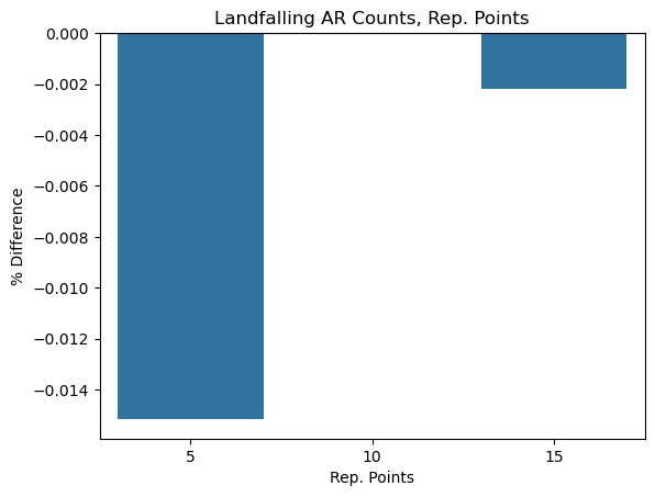

Takeaway: results seem fairly stable to perturbations of this parameter.

seed perturbations¶

Finally, we perturb the random seed. As there is a stochastic component to this algorithm since we randomly sample representative points from each identified spatial cluster, it is useful to see how sensitive our results are to random sampling.

seed_dict = {}
seed_dict['1111'] = load_catalog('epsspace0.5_epstime12_minpts5_nreppts10_seed1111.h5')
seed_dict['12345'] = baseline_df
seed_dict['2222'] = load_catalog('epsspace0.5_epstime12_minpts5_nreppts10_seed2222.h5')
seed_dict['3333'] = load_catalog('epsspace0.5_epstime12_minpts5_nreppts10_seed3333.h5')
seed_dict['4444'] = load_catalog('epsspace0.5_epstime12_minpts5_nreppts10_seed4444.h5')
seed_dict['5555'] = load_catalog('epsspace0.5_epstime12_minpts5_nreppts10_seed5555.h5')

res_df = process_cts(seed_dict)
res_df

# percent difference, expressed as a percentage of the total number of storms in baseline configuration
seed_percents = (res_df - res_df.loc['12345'])/res_df.loc['12345']
seed_percents

sns.barplot(data=seed_percents, x=seed_percents.index, y='landfalling', errorbar=None)
plt.title('Landfalling AR Counts, Random Seed')
plt.axhline(y=0, linestyle='-', color='black')
plt.xlabel('Seed')
plt.ylabel('% Difference');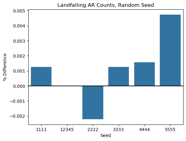

Takeaway: Results seem very stable to perturbations of the random seed, indicating that the randomness is not introducing too much variability into the numbers of ARs created.

All Together¶

We conclude by placing all of the above plots on shared axes so as to compare the sensitivity of our clustering output across the different hyperparameters, isolating which seem to play the most important role.

fig, axs = plt.subplots(2, 3, sharey=True)

sns.barplot(data=space_percents, x=space_percents.index, y='landfalling', errorbar=None, ax=axs[0,0])
axs[0,0].axhline(y=0, linestyle='-', color='black')
axs[0,0].set_title('Eps. Space')
axs[0,0].set_xlabel('')
axs[0,0].set_ylabel('% Difference');

sns.barplot(data=time_percents, x=time_percents.index, y='landfalling', errorbar=None, ax=axs[0,1])
axs[0,1].axhline(y=0, linestyle='-', color='black')
axs[0,1].set_title('Eps. Time')
axs[0,1].set_xlabel('')
axs[0,1].set_ylabel('');

sns.barplot(data=minpts_percents, x=minpts_percents.index, y='landfalling', errorbar=None, ax=axs[0,2])
axs[0,2].axhline(y=0, linestyle='-', color='black')
axs[0,2].set_title('Min. Pts.')
axs[0,2].set_xlabel('')
axs[0,2].set_ylabel('');

sns.barplot(data=rep_pts_percents, x=rep_pts_percents.index, y='landfalling', errorbar=None, ax=axs[1,0])
axs[1,0].axhline(y=0, linestyle='-', color='black')
axs[1,0].set_title('Rep. Points')
axs[1,0].set_xlabel('')
axs[1,0].set_ylabel('% Difference');

sns.barplot(data=seed_percents, x=seed_percents.index, y='landfalling', errorbar=None, ax=axs[1,1])
axs[1,1].set_title('Random Seed')
axs[1,1].axhline(y=0, linestyle='-', color='black')
axs[1,1].set_xlabel('Seed')
axs[1,1].set_ylabel('');

axs[1,2].set_axis_off()


fig.set_size_inches((10,6))
plt.tight_layout()
plt.savefig('../../output/plots/sensitivity_testing.png', dpi=300)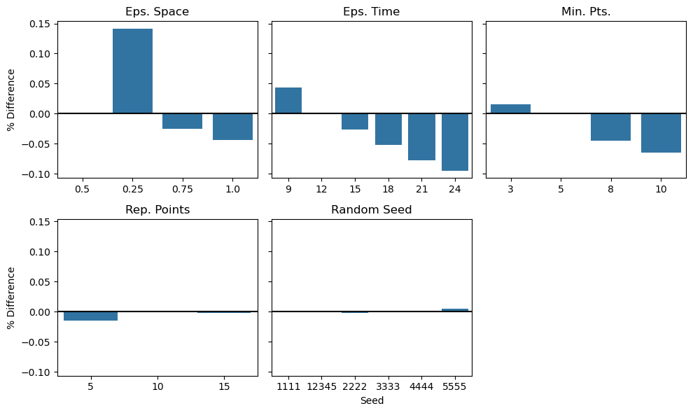

References¶

Maclennan, M. L., Lenaerts, J. T. M., Shields, C. A., Hoffman, A. O., Wever, N., Thompson-Munson, M., Winters, A. C., Pettit, E. C., Scambos, T. A., & Wille, J. D. (2023). Climatology and surface impacts of atmospheric rivers on West Antarctica. The Cryosphere, 17(2), 865–881. 10.5194/tc-17-865-2023
Birant, D., & Kut, A. (2007). ST-DBSCAN: An algorithm for clustering spatial–temporal data. Data & Knowledge Engineering, 60(1), 208–221. 10.1016/j.datak.2006.01.013

Hyperparameters Overview¶

epsilon_space perturbations¶

epsilon_time perturbations¶

minpts perturbations¶

n_rep_pts perturbations¶

seed perturbations¶

All Together¶

`epsilon_space` perturbations¶

`epsilon_time` perturbations¶

`minpts` perturbations¶

`n_rep_pts` perturbations¶