Aggregate Statistics Comparisons - Constructing Datasets of Antarctic AR Events

To further validate our catalog, in addition to ensuring we properly identified known storms presented in case studies, we also check that we are able to reproduce AR count statistics, by year and by geographic location, reported in the literature.

import numpy as np
import matplotlib.pyplot as plt
from matplotlib.patches import Polygon
import pandas as pd
import xarray as xr
import seaborn as sns
import os
import cartopy.crs as ccrs
import cartopy.feature as cfeature
import matplotlib.path as mpath
from scipy.stats import linregress
from huggingface_hub import login, hf_hub_download

from artools.attribute_utils import *
from artools.loading_utils import *

/home/jovyan/antarctic_AR_dataset/notebooks/quality_assurance

# loading up the ais and catalogs
ais_mask = load_ais()
df = load_catalog('epsspace0.5_epstime12_minpts5_nreppts10_seed12345.h5')
landfalling_df = df[df.is_landfalling]

# add in landfalling times and durations
landfalling_df['landfalling_duration'] = landfalling_df['data_array'].apply(compute_duration, ais_da=ais_mask)
landfalling_df['landfalling_start_date'] = landfalling_df['data_array'].apply(add_start_date, ais_da=ais_mask)
landfalling_df['landfalling_end_date'] = landfalling_df['data_array'].apply(add_end_date, ais_da=ais_mask)

Histograms of Landfalling Locations¶

We first reproduce Figure 1b of Synoptic and planetary-scale dynamics modulate Antarctic atmospheric river precipitation intensity using data from our catalog. For ease of comparison, we replot their figure with our own plotting code, with the same underlying data as in the original figure (provided by the authors).

To make this plot, we first write a function that, given an AR’s data array, finds all of the average longitudes across the $55^{\circ}$ S latitude for each time step the AR passes through.

def get_avg_landfall_lons(da, target_lat=-55):

    # force coordinates to be the same (avoid floating point errors)
    clean_lat = ais_mask.sel(lat=da.lat, method="nearest").lat
    clean_lon = ais_mask.sel(lon=da.lon, method="nearest").lon
    da = da.assign_coords(lat=clean_lat, lon=clean_lon)
    
    # subset time steps where AR is actively making landfall
    ais_mask_subset = ais_mask.sel(lat=da.lat, lon=da.lon)
    ais_storm_mask = da*ais_mask_subset
    landfall_times = da.time[ais_storm_mask.any(dim=['lat', 'lon'])]
    landfall_da = da.sel(time=landfall_times)

    da_lat = landfall_da.sel(lat=target_lat, method='nearest')
    mask = da_lat.astype(float)
    counts = mask.sum(dim='lon')
    
    # convert coordinates to radians and calculate Cartesian
    lat_rad = np.radians(da_lat.lat)
    lon_rad = np.radians(da_lat.lon)
    x = np.cos(lat_rad)*np.cos(lon_rad)
    y = np.cos(lat_rad)*np.sin(lon_rad)
    
    # calculate the average x and y only where the mask == 1
    avg_x = (x*mask).sum(dim='lon')/counts
    avg_y = (y*mask).sum(dim='lon')/counts
    
    avg_lon_rad = np.arctan2(avg_y, avg_x)
    avg_lon_deg = np.degrees(avg_lon_rad)
    
    avg_lon_deg = avg_lon_deg.where(counts > 0, np.nan)
    
    return avg_lon_deg

Then, we apply this function to all of the ARs and organize the average longitudes into a list, such that we have a list of average longitudes at each AR timestep.

mean_lons_list = [get_avg_landfall_lons(ar.data_array, target_lat=-55) for index, ar in landfalling_df.iterrows()]
all_mean_lons = np.concatenate([m.values for m in mean_lons_list])
# filter out NaNs (storms that never crossed 55 S)
clean_mean_lons = all_mean_lons[~np.isnan(all_mean_lons)]

We also load up the original longitude data used in the figure we are reproducing.

original_lons = pd.read_csv('../../input_data/reproducing_plots_data/original_centers.csv')
original_lons = np.array(original_lons.center_55)

fig, axs = plt.subplots(1, 3, figsize=(18, 6), subplot_kw={'projection': ccrs.Stereographic(central_longitude=0., central_latitude=-90.)})

ice_shelf_poly = cfeature.NaturalEarthFeature('physical', 'antarctic_ice_shelves_polys', '50m', edgecolor='none', facecolor='lightcyan')
ice_shelf_line = cfeature.NaturalEarthFeature('physical', 'antarctic_ice_shelves_lines', '50m', edgecolor='black', facecolor='none')

for ax in axs:
    ax.add_feature(ice_shelf_poly, linewidth=3)
    ax.add_feature(ice_shelf_line, linewidth=1, zorder=13)
    ax.coastlines(resolution='110m', linewidth=1, zorder=32)
    ax.set_extent([-180, 180, -90, -40], ccrs.PlateCarree())
    ax.grid(True, linestyle='--', color='gray', alpha=0.5)
    
    # Circular boundary
    theta = np.linspace(0, 2*np.pi, 100)
    center, radius = [0.5, 0.5], 0.5
    verts = np.vstack([np.sin(theta), np.cos(theta)]).T
    circle = mpath.Path(verts * radius + center)
    ax.set_boundary(circle, transform=ax.transAxes)
    ax.gridlines(alpha=0.5, zorder=33)

axs[0].set_title('(a) Original', pad=15, fontsize=20)
axs[1].set_title('(b) Replication', pad=15, fontsize=20)
axs[2].set_title('(c) Difference', pad=15, fontsize=20)

num_bins = 72
counts, bin_edges = np.histogram(clean_mean_lons, bins=num_bins, range=(-180, 180), density=True)
counts_orig, bin_edges_orig = np.histogram(original_lons, bins=num_bins, range=(-180, 180), density=True)

# calculate the difference (Original minus Replication)
counts_diff = counts_orig - counts

baseline_lat = -55
max_lat_stretch = 10 

global_max = max(counts.max(), counts_orig.max())

# ccale raw counts and original counts
scaled_heights = (counts / global_max) * max_lat_stretch
scaled_heights_orig = (counts_orig / global_max) * max_lat_stretch

# for difference, preserve the sign before scaling
scaled_diffs = (counts_diff / global_max) * max_lat_stretch

# drawing the polygons
for i in range(len(counts)):
    lon1, lon2 = bin_edges[i], bin_edges[i+1]
    lons = np.linspace(lon1, lon2, 10)
    
    # common elements
    baseline_lat_vec = np.full_like(lons, baseline_lat)
    
    # plot original (axs[0])
    if counts_orig[i] > 0:
        lat_top_orig = baseline_lat + scaled_heights_orig[i]
        top_edge_orig = np.column_stack((lons, np.full_like(lons, lat_top_orig)))
        bottom_edge_orig = np.column_stack((lons[::-1], baseline_lat_vec))
        verts_orig = np.vstack((top_edge_orig, bottom_edge_orig))
        
        poly_orig = Polygon(verts_orig, facecolor='lightgray', edgecolor='black', 
                            transform=ccrs.PlateCarree(), alpha=0.8, zorder=10)
        axs[0].add_patch(poly_orig)

    # plot replication (axs[1])
    if counts[i] > 0:
        lat_top = baseline_lat + scaled_heights[i]
        top_edge = np.column_stack((lons, np.full_like(lons, lat_top)))
        bottom_edge = np.column_stack((lons[::-1], baseline_lat_vec))
        verts = np.vstack((top_edge, bottom_edge))
        
        poly = Polygon(verts, facecolor='lightgray', edgecolor='black', 
                       transform=ccrs.PlateCarree(), alpha=0.8, zorder=10)
        axs[1].add_patch(poly)
        
    # plot difference (axs[2])
    # Now, lat_2 could be less than baseline_lat
    if scaled_diffs[i] != 0:
        lat_2 = baseline_lat + scaled_diffs[i]
        top_edge_diff = np.column_stack((lons, np.full_like(lons, lat_2)))
        bottom_edge_diff = np.column_stack((lons[::-1], baseline_lat_vec))
        verts_diff = np.vstack((top_edge_diff, bottom_edge_diff))
        
        # Keep colors for extra clarity: Coral (Positive), Cornflowerblue (Negative)
        diff_color = 'coral' if scaled_diffs[i] > 0 else 'cornflowerblue'
        
        poly_diff = Polygon(verts_diff, facecolor=diff_color, edgecolor='black', 
                            transform=ccrs.PlateCarree(), alpha=0.8, zorder=10)
        axs[2].add_patch(poly_diff)

plt.tight_layout()
fig.savefig('../../output/plots/reproduce_longitudinal_hist_directional.png', dpi=300, bbox_inches='tight')
plt.show()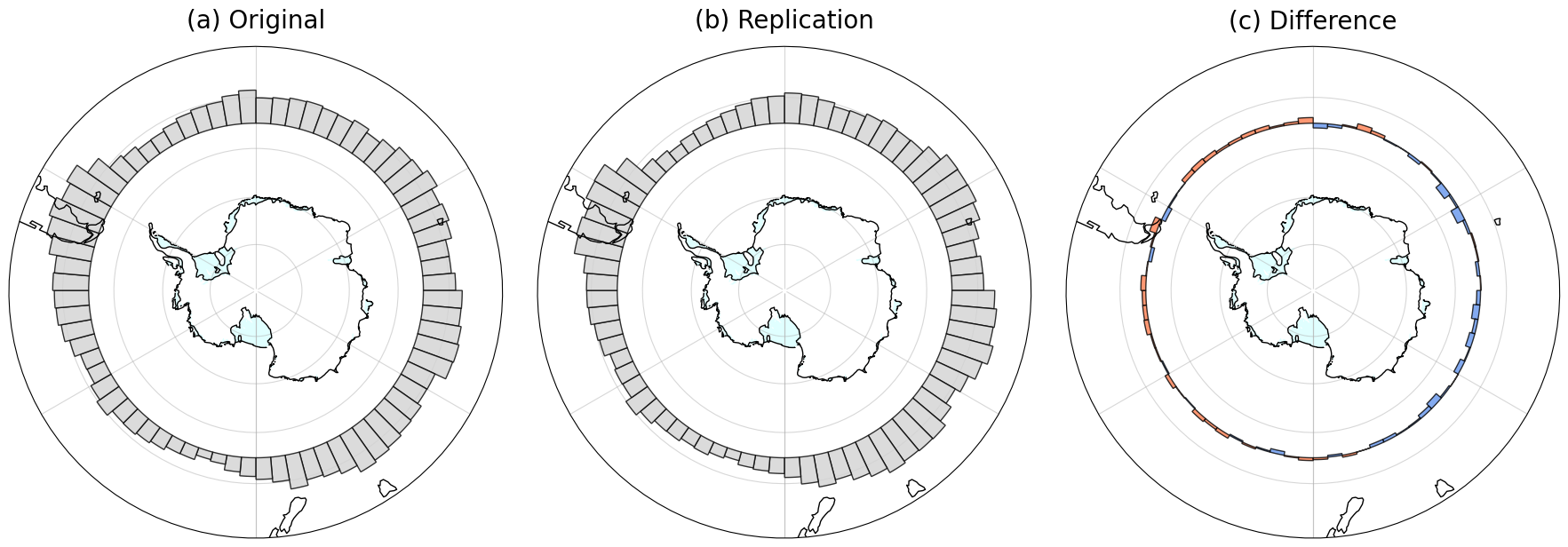

We see similarities in the distribution of average longitudes between our plot and the original. For instance, we see higher counts around longitudes near the Antarctic Peninsula, steady amounts across East Antarctic longitudes, and the lowest counts near the Ross Ice Shelf.

Durations and Counts in West Antarctica¶

Next, we seek to reproduce various statistics and figures from Climatology and surface impacts of atmospheric rivers on West Antarctica by Maclennan et al., which conducts an extensive analysis of AR landfall counts and durations in Marie Byrd Land and the Amnudsen Sea Embayment.

We first define two functions, one which determines if an AR falls at all within a spatial bounding box, and also for how many hours the storm spends in the the bounding box.

def is_in_region(da, lat_low, lat_high, lon_low, lon_high):
    in_region = da.where((da.lat <= lat_high) & 
                         (da.lat >= lat_low) & 
                         (da.lon <= lon_high) & 
                         (da.lon >= lon_low), drop=True).any().values
    return in_region

def duration_in_region(da, lat_low, lat_high, lon_low, lon_high):
    region_mask = da.where((da.lat <= lat_high) & 
                           (da.lat >= lat_low) & 
                           (da.lon <= lon_high) & 
                           (da.lon >= lon_low), drop=True)
    times = region_mask.time[region_mask.any(dim=['lat', 'lon'])]
    duration = (times.values[-1] - times.values[0]).astype('timedelta64[h]') + np.timedelta64(3, 'h')

    return duration

We count a storm as making landfall in Marie Byrd Land/Amundsen Sea Embayment if it intsersects $72.5^{\circ}$ S, between $150^{\circ}$ W and $80^{\circ}$ W. The duration of landfall is counted as the elapsed time between the first time it passes through the region defined by these longitudes and between $80^{\circ}$ S and $72.5^{\circ}$ S, and the last. We choose the coordinate $72.5^{\circ}$ S beceause this arc roughly corresponds to the coastline, and $150^{\circ}$ W and $80^{\circ}$ W as this range roughly covers the geographic region of interest. The original paper uses ARs defined up to $80^{\circ}$ S.

landfalling_df['in_MBL_ASE'] = landfalling_df['data_array'].apply(lambda x: is_in_region(x, -72.5, -72.5, -150, -80))
mbl_ase_storms = landfalling_df[landfalling_df.in_MBL_ASE]
mbl_ase_storms['duration_MBL_ASE'] = mbl_ase_storms['data_array'].apply(lambda x: duration_in_region(x, -80, -72.5, -150, -80))

We first seek to reproduce Figures 3a and 3b from Maclennan et al. (2023).

num_storms = mbl_ase_storms.groupby(mbl_ase_storms.landfalling_start_date.dt.year, as_index=False).size()
num_storms = num_storms[num_storms.landfalling_start_date <= 2020]

x = num_storms['landfalling_start_date']
y = num_storms['size']
slope, intercept, r_value, p_value, std_err = linregress(x, y)
sns.lineplot(data=num_storms, x='landfalling_start_date', y='size', alpha=0.5)
sns.scatterplot(data=num_storms, x='landfalling_start_date', y='size')
sns.regplot(data=num_storms, x='landfalling_start_date', y='size', 
            scatter=False, color='red', line_kws={'linestyle': '--'}, ci=None)

plt.title('Number of Storms in Marie Byrd Land + Amundsen Sea Embayment')
plt.xlabel('Year')
plt.ylabel('Number of Storms')
text_box = f"+{slope:.2f} $\\pm$ {std_err:.2f} storms/year"
plt.text(0.05, 0.90, text_box, 
         transform=plt.gca().transAxes, 
         fontsize=11, color='black')
plt.grid()
plt.savefig('../../output/plots/mbl_ase_counts.png', dpi=300)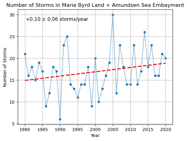

We find several similarities between our reproduction of the plot and the original, including downward spikes at 1990, 2001, and 2009, and upward spikes in 1992, 2005, and 2014. Further, we find an upward trend of $0.10 \pm 0.06$ additional storms per year and the original paper reports $0.12 \pm 0.06$ .

Further, the original paper reports a yearly average of $17 \pm 5$ AR events during this period. Rounding to the nearest integer, we compute the same average and standard deviation.

float(num_storms['size'].mean())

16.878048780487806

float(num_storms['size'].std())

4.995973988879544

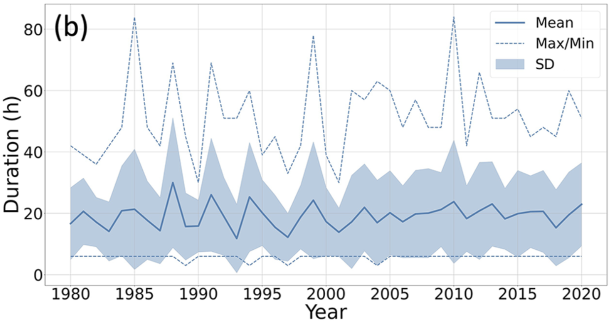
Lastly, we seek to reproduce Figure 3b.

mbl_ase_storms_mean_durations = mbl_ase_storms.groupby(mbl_ase_storms.landfalling_start_date.dt.year).duration_MBL_ASE.mean()/np.timedelta64(1, 'h')
mbl_ase_storms_sd_durations = mbl_ase_storms.groupby(mbl_ase_storms.landfalling_start_date.dt.year).duration_MBL_ASE.std()/np.timedelta64(1, 'h')
mbl_ase_storms_plussd_durations = mbl_ase_storms_mean_durations + mbl_ase_storms_sd_durations
mbl_ase_storms_minussd_durations = mbl_ase_storms_mean_durations - mbl_ase_storms_sd_durations
mbl_ase_storms_max_durations = mbl_ase_storms.groupby(mbl_ase_storms.landfalling_start_date.dt.year).duration_MBL_ASE.max()/np.timedelta64(1, 'h')
mbl_ase_storms_min_durations = mbl_ase_storms.groupby(mbl_ase_storms.landfalling_start_date.dt.year).duration_MBL_ASE.min()/np.timedelta64(1, 'h')

durations_df = pd.concat({'mean': mbl_ase_storms_mean_durations, 
                          'plus_sd':mbl_ase_storms_plussd_durations, 
                          'minus_sd': mbl_ase_storms_minussd_durations, 
                          'max': mbl_ase_storms_max_durations, 
                          'min': mbl_ase_storms_min_durations}, axis=1)
durations_df = durations_df.reset_index()

plt.figure(figsize=(8, 4))
plt.grid(zorder=0)
sns.lineplot(data=durations_df, x='landfalling_start_date', y='max', color='darkblue', label='Max/Min', linestyle='dotted')
sns.lineplot(data=durations_df, x='landfalling_start_date', y='min', color='darkblue', linestyle='dotted')

plt.fill_between(
    durations_df['landfalling_start_date'], 
    durations_df['minus_sd'], 
    durations_df['plus_sd'], 
    color='darkblue', 
    alpha=0.1, 
    label='±1 SD',
    zorder=2
)

sns.lineplot(data=durations_df, x='landfalling_start_date', y='mean', label='Mean', zorder=3)
sns.scatterplot(data=durations_df, x='landfalling_start_date', y='mean', zorder=4)

plt.title('MBL + ASE Storm Durations over Time')
plt.xlabel('Year')
plt.ylabel('Duration (Hours)')
plt.legend(loc='upper left')
plt.savefig('../../output/plots/mbl_ase_durations.png', dpi=300)

plt.show()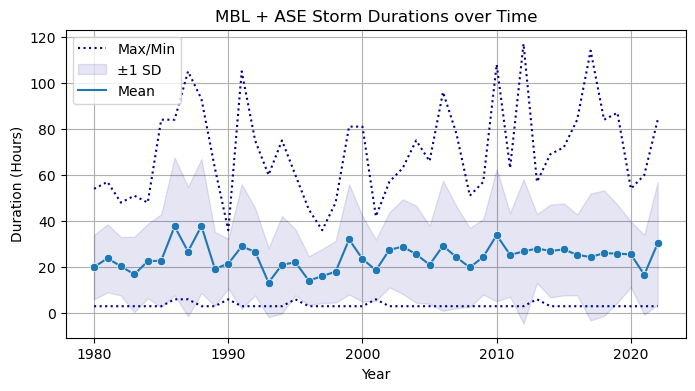

We see similarities with the original figure, including max duration upward spikes at 1987, 1991, 2010, and 2012, and a notable downward spike at 1990.

hourly_durations = mbl_ase_storms.duration_MBL_ASE.dt.total_seconds()/3600
hourly_durations.mean()

np.float64(24.39693593314763)

hourly_durations.std()

np.float64(20.23019110538663)

References¶

Baiman, R., Winters, A. C., Pohl, B., Favier, V., Wille, J. D., & Clem, K. R. (2024). Synoptic and planetary-scale dynamics modulate Antarctic atmospheric river precipitation intensity. Communications Earth & Environment, 5(1). 10.1038/s43247-024-01307-9
Maclennan, M. L., Lenaerts, J. T. M., Shields, C. A., Hoffman, A. O., Wever, N., Thompson-Munson, M., Winters, A. C., Pettit, E. C., Scambos, T. A., & Wille, J. D. (2023). Climatology and surface impacts of atmospheric rivers on West Antarctica. The Cryosphere, 17(2), 865–881. 10.5194/tc-17-865-2023